Composing Value Functions in Reinforcement Learning

Introduction

In this post, we look to answer the following question: given a set of existing skills, can we compose them to produce novel behaviours? For example, imagine we have learned skills like running and jumping. Can we build more complex skills by simply combining them in interesting ways? Of course, it is likely that there are many ad-hoc ways to do this, but it would be really nice if we could do it in a way that is both provably correct and that requires no further learning.

To illustrate what we’re after, we use pretrained skills generated by DeepMimic [Peng, 2018]. As we can see, in the first two animations below our agent has learned to backflip and spin. But if we try to combine these skills together (in this case, by taking the maximum of the policy network output), we get complete bupkis! The question is: is there some way we can make this work?

Attempting to compose two skills - backflips and spins - results in an agent that can injure itself optimally.

Unsurprisingly, the answer is “yes”. More surprisingly, perhaps, is that this was shown many years ago! Under the framework of Linearly-solvable Markov Decision Processes (LMDPs), Todorov [2009] demonstrated that we can take two optimal LMDP value functions and combine them together to solve a composite task optimally. Unfortunately, LMDPs are quite restrictive, and it’s unclear how we can extend them beyond the tabular case.
In the rest of this post, we’ll look at how we can achieve the same kind of composition in a more scalable way.

Entropy-regularised RL

Entropy-regularised RL extends standard RL by appending a additional term that penalises our current policy \(\pi\) for being too far away from a reference policy \(\bar{\pi}\). The reference policy can be any policy—an expert policy, human demonstration, etc — but the most common is simply the uniform random policy. Whatever the case, introducing this penalty results in a value function defined as

\[V^\pi(s)=\mathbb{E}_\pi \left[ \sum\limits_{t =0}^\infty r(s_t, a_t) - \tau \text{KL}[\pi_{s_t} || \bar{\pi}_{s_t} ] \right],\]

where \(\tau > 0\) is a temperature parameter.

It turns out that we can define equivalent Bellman operators for the above definition and find optimal value functions using value or policy iteration. We will look at the undiscounted case where—after lots of blood, sweat and maths—the same convergence results hold. Great, so we can solve undiscounted, entropy-regularised MDPs for the optimal value function. But how exactly does this help us?

The reason composition is achievable in LMDPs is because of the linear part. We can’t compose value functions normally because the Bellman equation is non-linear (on account of the \(\max\) operator). In LMDPs, the relaxations produce a linear Bellman operator (hence the name), and so composition all works out. It turns out that the same thing happens in entropy-regularised RL, where the new Bellman equation \(\mathcal{L}\) is given by

\[[\mathcal{L}V^\pi](s) = \tau \log \int_\mathcal{A} \exp(Q^\pi(s, a) / \tau) \bar{\pi}_s(da).\]

We call this the “soft” Bellman operator, because it is a smooth approximation to the \(\max\) operator. Importantly, note that it is a linear function of the exponentiated \(Q\)-value, which is exactly the same as the LMDP case.

Entropy-regularised composition

Because entropy-regularisation linearises the Bellman equation, it should come as no surprise that we can achieve LMDP-like composition. We will consider a family of tasks that have the same deterministic transition dynamics and differ only in reward functions. We also need to restrict the reward functions (as in LMDPs) so that it differs only when entering terminal states. For all non-terminal states, the rewards must be the same. Though restrictive, we can still make use of sparse rewards. For instance, an agent can receive \(-1\) everywhere. and \(+1\) for entering the current task’s terminal states.

If we let \(\mathbf{r}\) be a vector of all tasks’ reward functions, and \(\mathbf{Q}^*\) the corresponding optimal \(Q\)-value functions, then for a task with reward function

\[r(s, a) = \tau \log (||\exp(\mathbf{r}(s,a)/\tau)||_\mathbf{w}),\]

the optimal \(Q\)-value function is

\[Q^*(s, a) = \tau \log (||\exp(\mathbf{Q}^*(s,a)/\tau)||_\mathbf{w}).\]

Semantically, this corresponds to doing –OR– composition. Recall that \(\text{logsumexp}\) is a smooth version of the \(\max\) operator. Recall even further back truth tables, where binary OR is simply the maximum of two Boolean variables. Thus if we’ve learned to solve tasks A and B separately, we can immediately solve A–OR–B without further learning. Note that we only need the base \(Q\)-value functions, which can be learned through any (deep) RL method.

Multimodal composition

One advantage of this approach is for multi-objective environments. Imagine an agent needed to reach one of two equidistant goals as quickly as possible. If we simply learned from scratch, it’s more than likely that the agent’s policy would collapse to only one of the two. While there are approaches to overcome this collapse (e.g. Haarnoja 2017), they’re brittle, hard to tune and have no guarantees. Here instead we can simply learn to reach each goal individually, and then compose to produce a truly multimodal policy.

To show this, we create an environment called BoxMan, where a character must move around collecting objects. There are crates and circles, each of which is either blue, purple or beige. The state space is the current RGB frame, and we use deep Q-learning to solve a set of base tasks.

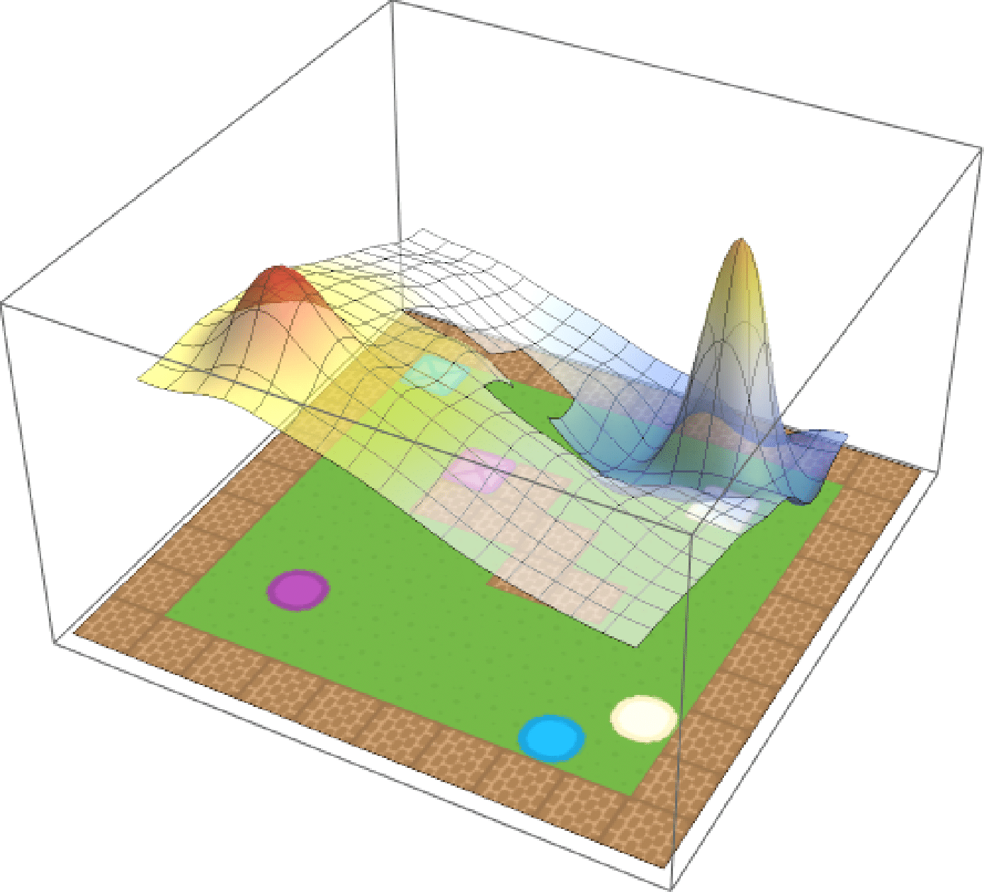
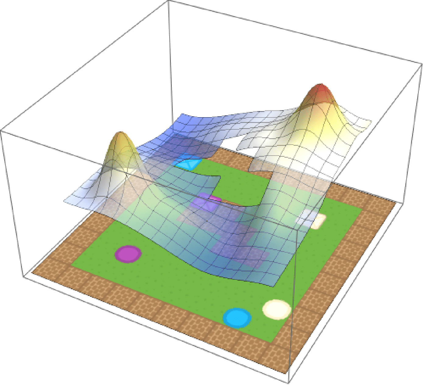
To illustrate multimodality, we train the agent to pick up purple circles and beige squares separately and compose the resulting value functions as per our equation. The composed value function, illustrated below, clearly capture the semantics of PurpleCircle–OR–BeigeSquare.

A multimodal, entropy-regularised value function created by composing the constituent value functions together.

Weighted composition

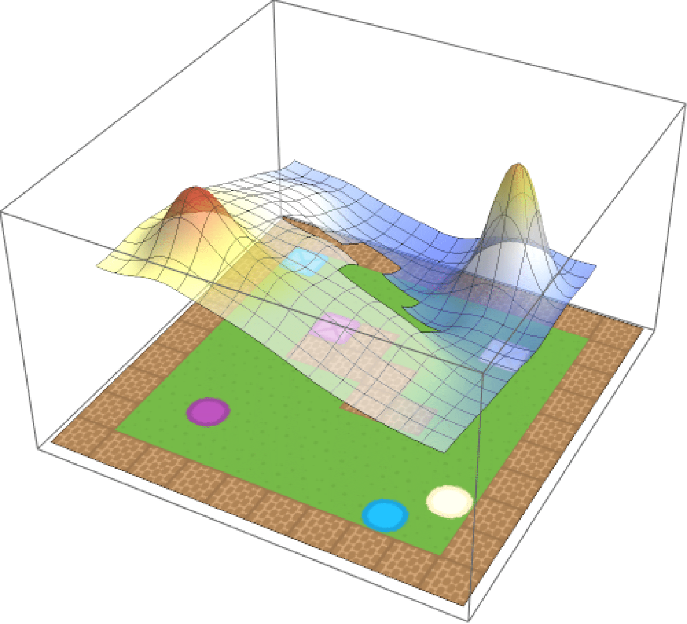
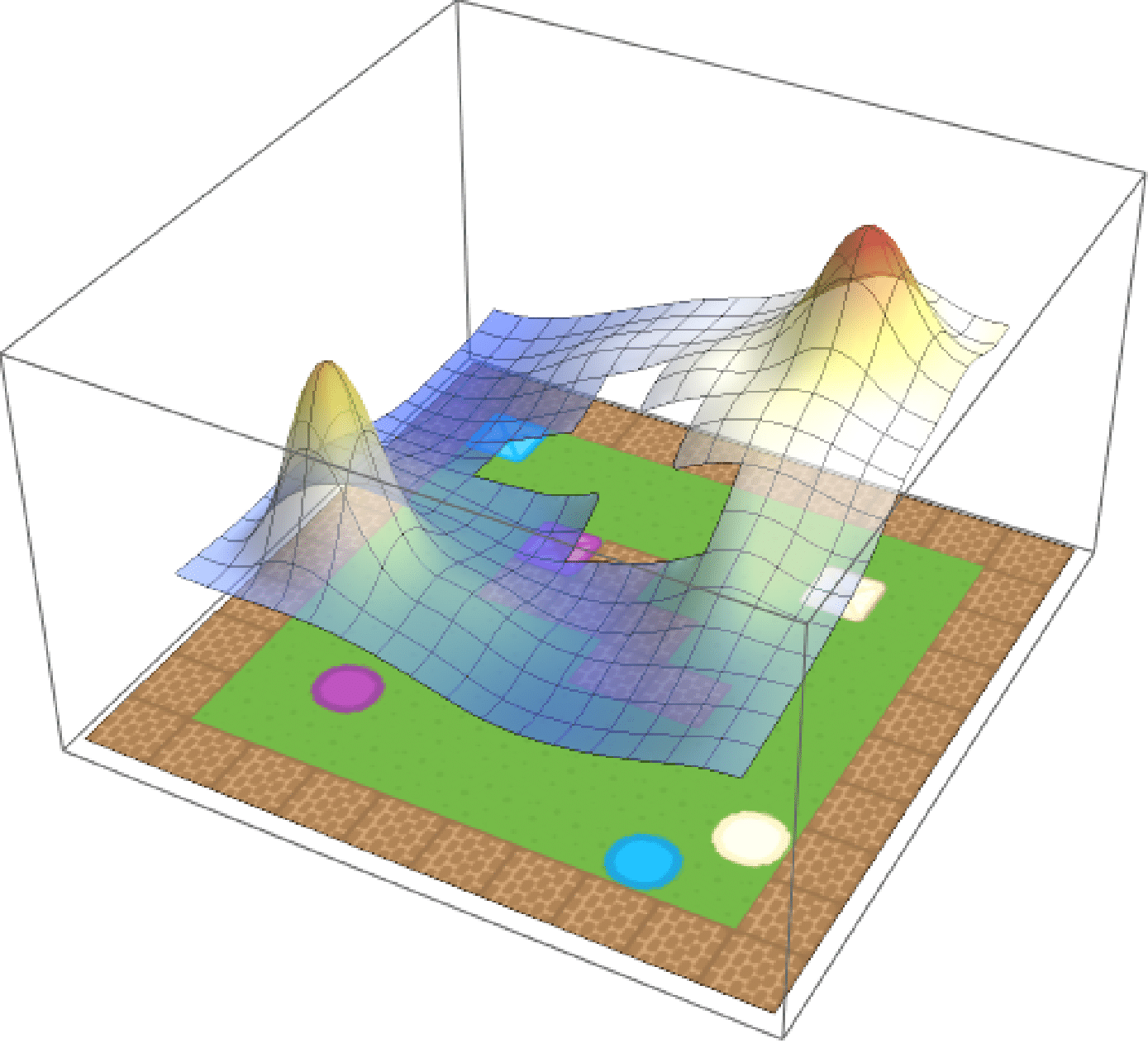
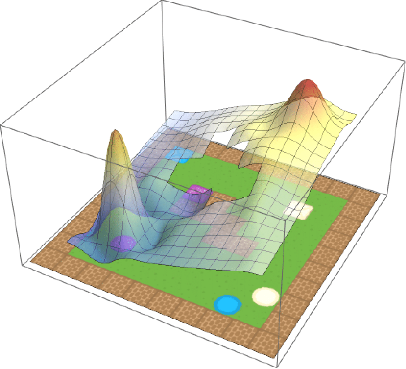
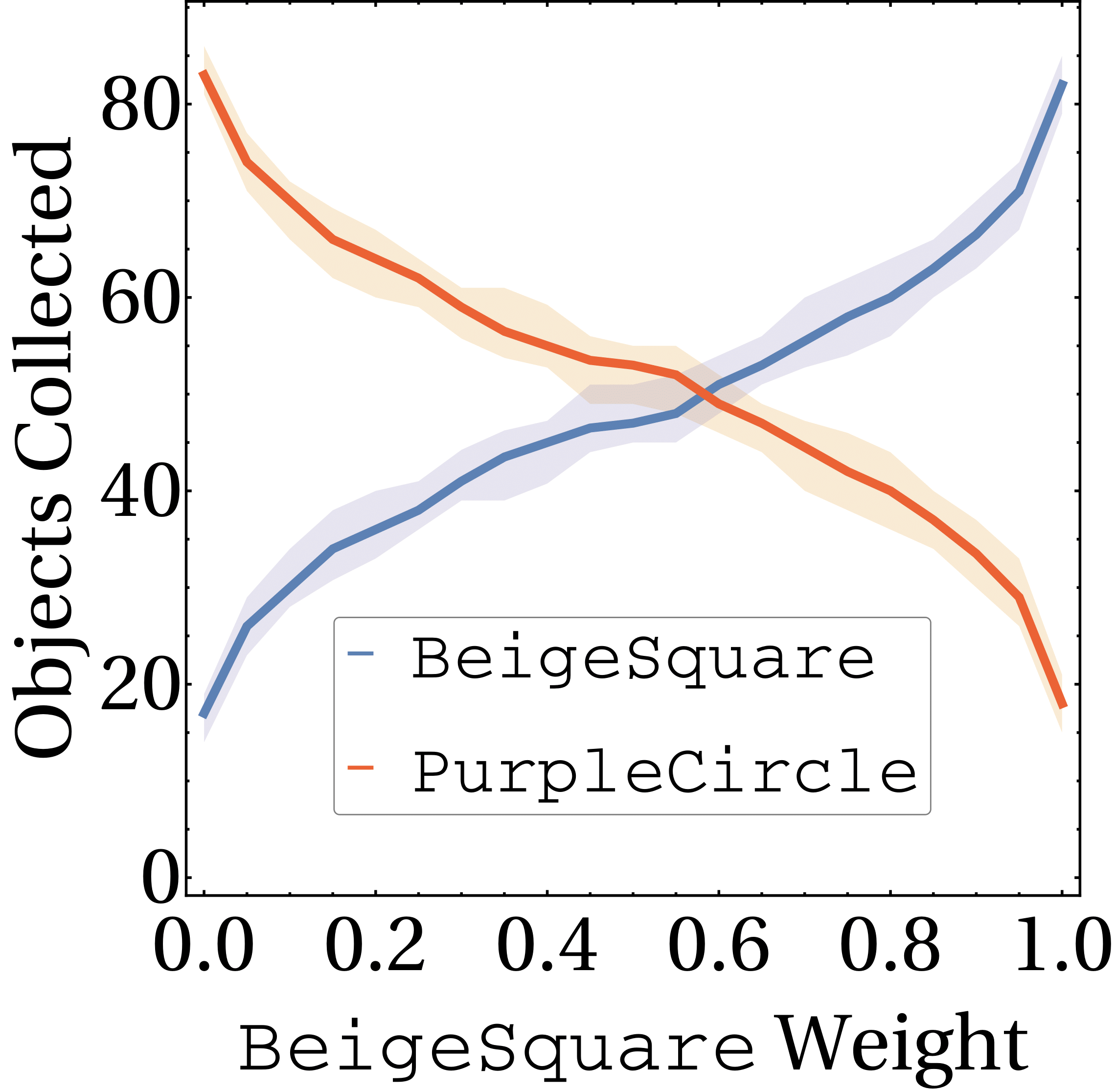
Eagled-eyed readers will have noticed that the formula for composition contained a weighted norm. These weights \(\textbf{w}\) are arbitrary and can be used to assign priority to different tasks.If we care about purple circles and beige squares equally, we can simply set \(\textbf{w} = (0.5, 0.5)\). But maybe we prefer purple circles, in which case we can update out weights accordingly (e.g. \(\textbf{w} = (0.75, 0.25)\)). We show the effect of modifying the weights in the below, where the weight for beige crates is increased from \(0\) to \(1\) over time.

From left to right, increasing the weight assigned to the beige crate modifies the composed value function. As the weight increases, the value function encourages the collection of beige crates. The last graph shows how the number of the different collected objects changes as a function of weights. As the beige crate weight tends to 1, the number of collected beige crates increases. Similarly, as it tends to 0, the number decreases.

Composition in standard RL

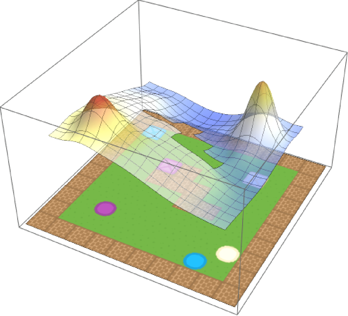
We’ve talked so far only about entropy-regularised RL, but what of the standard case? To put more concretely, what happens when \(\tau \to 0\) and the penalty term disappears. Turns out that it’s exactly what you would imagine—all the soft approximations to \(\max\) simply become \(\max\). Now, for the composite task with reward function

\[r(s, a) = \max\mathbf{r},\]

the optimal \(Q\)-value function is

\[Q^*(s, a) = \max\mathbf{Q}^*.\]

We show this by learning base tasks corresponding to collecting purple and blue objects, and then composing them as above. The composed value function and agent behaviour is shown below.

On the left, the agent has learned to collect blue objects, while in the middle it has separately learned to collect purple ones. These value functions can be composed to produce multimodal behaviour, collecting either blue or purple objects in the rightmost animation.

Other forms of composition

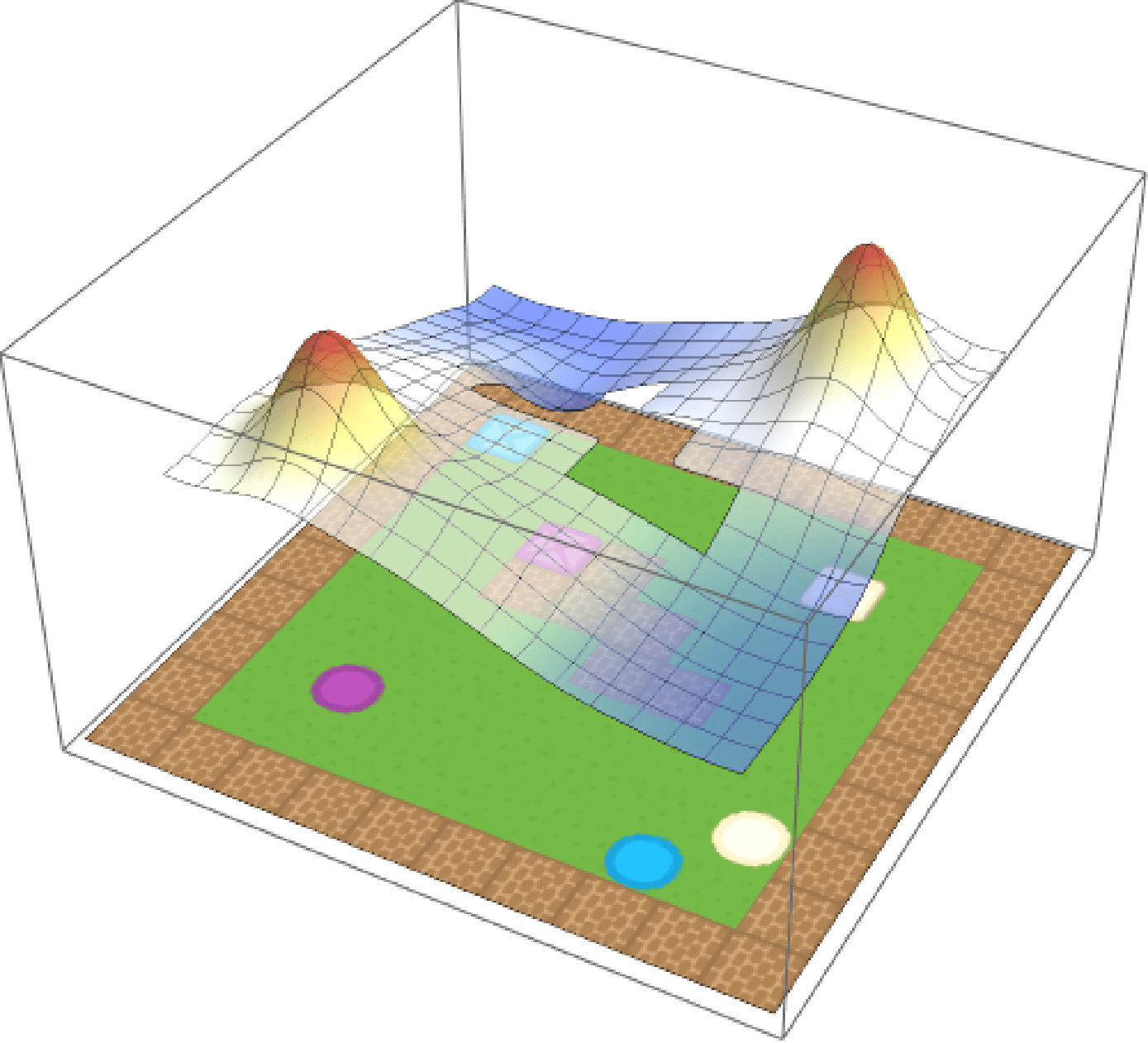
We finally show that other kinds of composition seem to be achievable empirically. Haarnoja [2018] suggests using the average reward to approximate –AND– composition in entropy-regularised RL. We find that this works pretty well in standard RL too, by simply averaging the base \(Q\)-value functions. Here we show behaviour for the Blue–AND—Crate task.

Collecting blue objects and crates in the first two animations respectively. These are averaged to collect blue crates approximately optimally (right frame).

Lastly, if the environment is amenable, it’s possible to chain base tasks one-after the other. By considering the standard –OR– composition, but then allowing the agent not to terminate at the goal states, we can approximate temporal composition. Here we first learn a value function to collect each colour. By executing the composed value function, we can let it run and it will collect all the objects in the environment.

Examples of the agent using composition to collect all objects.

Conclusion

We showed how to achieve composition in a way that scales to high-dimensional problems. This can be achieved in both standard and entropy-regularised RL. As a result, an agent can (automatically and for free) leverage existing skills to build new ones, resulting in a combinatorial explosion in the agent’s abilities. We believe this will be an important aspect in achieving true lifelong-learning agents.

References

[Todorov 2009] E. Todorov. Compositionality of optimal control laws. In Advances in Neural Information Processing Systems, 2009.
[Haaronoja 2017] T. Haarnoja, H. Tang, P. Abbeel, and S. Levine. Reinforcement learning with deep energy-based policies. In International Conference on Machine Learning, 2017.
[Haarnoja 2018] T. Haarnoja, V. Pong, A. Zhou, M. Dalal, P. Abbeel, and S. Levine. Composable deep reinforcement learning for robotic manipulation. In International Conference on Robotics and Automation, 2018.
[Peng 2018] X. Peng, P. Abbeel, S. Levine, and M. van de Panne. DeepMimic: Example-Guided Deep Reinforcement Learning of Physics-Based Character Skills. In Transactions on Graphics, 2018.